Deriving Equations of Motion (Graphical Method)

🌟 Introduction to Equation of Motion

Ever wondered how those magical equations of motion were discovered? The secret lies in graphs! By using simple geometry on velocity-time graphs, we can derive these powerful equations. It’s like solving a puzzle where shapes reveal the secrets of motion! 🧩📐

📸 Velocity-Time Graph Illustration

📚 Key Concepts – Derivation of Motion Equations

🔹 Derivation of First Equation:

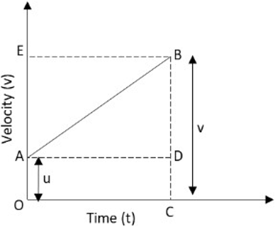
Consider the velocity-time graph of an object that moves under uniform acceleration as shown in the figure

From this graph, we can see that initial velocity of the object (at point A) is u and then it increases to v (at point B) in time t.
The velocity changes at a uniform rate a.
As shown in the figure, the lines BC and BE are drawn from point B on the time and the velocity axes respectively, so that the initial velocity is represented by OA, the final velocity is represented by BC and the time interval t is represented by OC. BD = BC – CD, represents the change in velocity in time interval t.

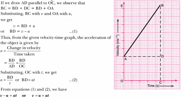
From the velocity-time graph:

🔁 Rearranging: v = u + at

🔹 Derivation of Second Equation:

s = ut + ½at²

From the velocity-time graph:

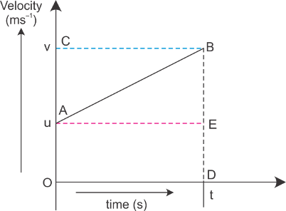
Displacement = Area under the graph = Area of trapezium OABC
Area of rectangle = u × t
Area of triangle = ½ × base × height = ½ × t × (v – u)
Since (v – u) = at ⇒ Triangle area = ½ × t × at = ½at²

📐 Total Distance: s = ut + ½at²

🔹 Derivation of Third Equation:

From the velocity-time graph:

v² = u² + 2as

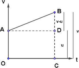
Displacement, s = Area of trapezium = ½ × (u + v) × t
From 1st equation: t = (v – u) / a
Substitute in s = ½ × (u + v) × (v – u) / a
⇒ s = (v² – u²) / 2a

🔁 Rearranging: v² = u² + 2as